Overview

• Cost starts in the low hundreds of dollars per vehicle in quantity

• Very small and low power consumption vehicle electronics package

• Ranging precision of 1.5cm typical. Position fixes of <10cm accuracy possible.

• Operating distance up to about 1000m

• Supports simultaneous navigation by an unlimited number of vehicles

• Passive operation. No acoustic emissions by the vehicle

• Many possible baseline configurations, including long baseline (LBL) and short baseline (SBL)

Background

Southstar is an underwater positioning system architecture that was originally developed for robotic under-the-ice exploration in Antarctica. The systems can be deployed in many different configurations, including for vehicle tracking and for autonomous vehicle navigation. When used as a passive acoustic position sensor, Southstar is in particular useful for small and swarming AUV.

In this configuration, Southstar vehicle electronics pick up the signals from one or several baseline stations that form the reference for navigation. By obtaining the precise distance from these baseline stations, the data from the position sensor is used to compute the precise vehicle position. The precision of the individual range measurements is on the order of 1.5cm. This ranging precision supports 3D position fixes with an accuracy of better than 10cm. However, 3D positioning accuracy depends on the deployment configuration of the baseline stations. Longer baselines result in better geometry and thus more accurate position fixes.

The passive operation of the acoustic position sensor keeps the package small and power consumption low. It also means that an unlimited number of vehicles can use the signals from the baseline network simultaneously without interfering with each other.

Vehicle Electronics

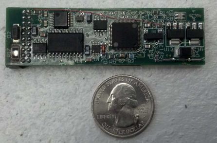
 The vehicle electronics are based on the EM-41 electronics module. The module measures 76mm x 22mm (3” x 0.85”) and consumes 16mA, accepting a supply voltage from 6V to 16V. Thus, at 6V supply, power consumption is about 100mW. Each module implements a single sonar channel. In most cases, one module is used for each baseline station in the configuration. The modules are configured and provide their data through simple text commands. Data transfer is via a RS-485 serial interface. Several EM-41 can share a twisted wire pair to form a party line. The EM-41 operate in slave mode, i.e. they respond to commands from a host processor.

The EM-41 module’s principal function is to measure the time of arrival (TOA) of signals from the baseline station. Depending on the synchronization scenario, either the distance to the baseline station or a pseudo-distance to the baseline station can be computed from the TOA. Computing actual 3D positions requires a position solver. This software may be implemented on the AUV’s host computer. Another option is the use of the CMR-41 carrier board. This board hosts four EM-41 modules and a processing engine that runs the position solver. The overall assembly measures 178mm x 58mm x 19mm (7” x 2.3” x 0.75”).

Clock Synchronization Options and Baseline Configurations

Southstar is based on one-way acoustics, in contrast to transponder systems that use an interrogate-and-reply cycle. In navigation sensor mode, the baseline stations ping and the vehicle stations listen for pings. There are several options to time synchronize the array in order to obtain either direct range measurements based on signal run time, or ‘pseudoranges’ [1]. For illustration, one example (in this case with divers instead of vehicles using the system to navigate) is shown below. The fixed baseline station (A) are linked via cable to surface buoy (B). The buoy provides clock synchronization through the GPS timing signal (1PPS). The diver stations (C) are not clock synchronized. The diver stations operate in passive mode, computing pseudoranges from the signals received from the baseline stations. At least four baseline stations are required; and position fixes also incorporate depth sensor readings from the diver station.

 In many AUV applications, the use of surface buoys to GPS time synchronize the baseline stations is not realistic. Several alternate clock synchronization options are possible:

1. The baseline stations are cabled together to form a short baseline (SBL) array. One baseline station is configured to operate as the clock transmitter (master station); the other baseline stations operate as clock receivers. Thus, all baseline stations are synchronized to the master station.

2. The EM-41 module includes a temperature compensated crystal oscillator (TCXO) with a stability of +/- 100 ppb. Based on a GPS timing signal received before each baseline station is submerged, the clocks of all baseline stations are synchronized and the oscillators are calibrated. Following submersion, the TCXO frequency stability limits drift (cumulative ranging error) to about +/- 0.5m per hour.

3. External synchronization through a chip scale atomic clock (CSAC) such as Microsemi Corps. SA-45 is available. With a stated stability of +/- 0.5 ppb, the cumulative ranging error is limited to +/- 0.0027m per hour

Baseline Length and its Relation to Positioning Accuracy

For geometric reasons, the length of the baseline (i.e. separation of the baseline stations) affects the accuracy of available position fixes. In the ideal ‘long baseline’ (LBL) case, the baseline stations are placed in the corners of the operating area. In this case, the limit of the position fix accuracy (on account of ranging precision and geometry alone) is the ranging precision multiplied by √2. For example, assuming a Southstar ranging precision of 1.5cm, then geometry will limit position fix accuracy to about 2.1cm. (note: other factors such as sound speed estimation errors and signal path distortions may add significant or dominant additional errors).

 

 

Field Performance Review

Ranging precision is a limiting factor for positioning accuracy with a Southstar sensor. Figure 2A above shows accuracy available with 1.5cm ranging precision, and figure 2B with a 10cm ranging precision assumption.

Short distance ranging precision

Figure 3 below shows results of a short-range ranging precision test. Four TLT-32 baseline stations (which are built around the EM-41 module), were arranged in an approximate rectangle configuration measuring 3.5m x 4.5m. The location was a floating dock in a Marina; i.e. an area with significant reverberations. The baseline stations were lowered over the side of the dock to a depth of about 2m. The configuration was static, so that repeat ranging should result in the same distance between any two stations on each measurement. The standard deviation of the measurements was from 0.2cm for Range #2 (most precise) to 1.8cm for Range #1 (least precise). The average of the standard deviation of the six range measurements was 1.0cm. These numbers establish the Southstar system limit for ranging precision.

 Figure 3: Short-distance ranging precision at a floating dock

 

Long distance ranging precision

The above test was for very short ranges. In general, one would expect some degradation of ranging precision over long distances. This may be in shallow waters for example owing to distortions of the signal due to multi-path propagation. Or, it may be due to the relative greater strength of noise in a weak signal environment. We do not have data for an equivalent long-distance static test. However, snippets of ranging from Southstar use with the SCINI ROV in Antarctica provide rough alternative. In this case, the ROV was never completely still, but there were periods where it was drifting slowly and one or another of the ranges was relatively static. The range measurements were from a TLT-3 pinger (EM- 41 electronics) tied to the ROV umbilical close to the vehicle, to four FRF-2 baseline stations including also TLT-32 acoustic units (with EM-41 electronics) lowered through holes in the sea ice. Water depth was from 17m to 50m, with the ROV generally operating near the bottom. The baseline stations were lowered to about 2m below the ice. Operating frequency 33.8kHz.

 

 Figure 6: Jitter (ΔRange) for B1, B2, B3, B4 Excerpts

The jitter for the long distance ranging experiment was computed as the average of |Rn – Rn-1| where Rn and Rn-1 are two successive range measurements. This simple metric overestimates the jitter because actual range changes as the ROV is drifting show up as part of the jitter. So, it might be considered a worst-case scenario. The results are:

Ranging from ROV to Baseline Station	Median Distance (m)	Average Jitter (cm)
B1	55	8.6
B2	154	5.6
B3	245	16.9
B4	209	8.5

 Table 1: Ranging jitter at various distances.

 The degraded ranging precision at longer distances approximately correlates with experience values. We consider it likely however that deep-water scenarios will show higher precision due to less multipath propagation.

Figure 7: SCINI ROV under the ice, with TLT-3 tracking pinger.

 

 

Sonar Transducer Options

The Southstar system can be configured for compatibility with various sonar transducers. Desert Star’s standard operating bands are 34kHz-42kHz, 16kHz-24kHz and 8kHz-16kHz.

 Lower frequency transducers provide greater range due to lower absorption losses. But, precision is less at lower frequencies, while size and cost is generally higher.

FREQUENCY RANGE	APROX. FREQUENCY SPECIFIC RANGING PRECISION LIMIT (theoretical limit)	APPROX. RANGE LIMIT WITH 192dB TRANSMITTER, 'MODERATE NOISE' 110dB DETECTION THRESHOLD AND 12dB FADING MARGIN
8kHz-16kHz (absorption 2dB/km)	+/- 3cm RMS	2000m
16kHz-24kHz(absorption 4dB/km)	+/- 1.8cm RMS	1500m
34kHz-42kHz(absorption 8dB/km)	+/- 1.0cm RMS	1100m

 The ceramic transducers shown here are relatively expensive. A better option for a passive Southstar position sensor is probably a sonar transducer based on piezoelectric film. Piezoelectric film is very inexpensive and can be bonded onto various substrates. The film is only suitable for receive mode, not transmit mode.

Desert Star Systems is scheduled to develop and support piezoelectric film based sonar transducer solutions in 2013, as these devices are now needed for several projects.

Southstar Passive Acoustic Position Sensor Specification Summary

Maximum practical range:Approx. 1100m-2000m depending on frequency selection in moderate ambient noise conditions. Shallow water propagation tends to be limited by multi-path / shadowing effects. Experience values are 25x depth for reliable operation, 50x depth typical and 100x depth under favorable conditions.

Positioning accuracy:Centimeter range to tens of meters depending on baseline geometry and distance. See figure 2.

Baseline stations:At least three needed in spherical mode (all stations synchronized). At least four stations in hyperbolic mode (vehicle station not synchronized to baseline stations)

Station synchronization options:

1. Per GPS 1PPS signal if a wired link to a surface GPS receiver is available

2. Baseline stations wire-synchronized to each other

3. Vehicle station not synchronized (hyperbolic mode / pseudorange measurements)

4. Vehicle station synchronized with EM-41 precision clock. Drift about 0.2-0.6ppm, Range measurement drift 1m-3m per hour

5. Vehicle station uses external very high precision clock oscillator with <0.01ppm drift. Range measurement drift is <0.05m per hour.

Power requirements: 6V-16V supply 16mA for single-channel system, 200mA for four-channel system with position solver

[1]:Pseudoranges are ranges that include an unknown but common error due to an unknown clock offset of the receiver vs. the signal transmitter. Pseudoranges are used when a receiver, such as on a free swimming vehicle, cannot be time synchronized to the baseline stations with sufficient accuracy. The baseline stations themselves must be time synchronized, either by using a cabled system where one baseline station serves as the clock transmitter and the other stations as clock receivers. Or, by using a surface buoy with a GPS receiver to obtain precision 1PPS timing. The pseudorange concept is explained on Wikipedia: http://en.wikipedia.org/wiki/Pseudorange